Weighted survey means with rstats

The following simple example will use European Social Survey (ESS) integrated datafile in order to plot unweighted and weighted distribution of the generalized trust variable (ppltrst).

TLDR; There are no significant differences between weighted and unweighted distribution of generalized trust among V4 countries.

The underlying codes demonstrate how to use srvyr and dplyr to work together on survey data. R can be difficult when it is about weighted sample data. Although survey package has been around quite long, its usage is not really straightforward. Advanced knowledge of survey sampling and R’s formula syntax¹ are must-haves. Nevertheless, survey is particularly useful for analyses of complex sampling design’s (eg. multi-staged cluster sample). Srvyr adds to it some useful features that fits well into tidyverse philosophy². For a detailed comparison with survey see this vignette at CRAN.

More to read:

1. Weighting European Social Survey Data
2. Federico Vegetti: Survey Weights with R
3. Kieran Healy: Data Visualization. (See. Chapter on “Plots from complex surveys”)
4. Thomas Lumley. 2010. Complex Surveys: A Guide to Analysis Using R
5. Webinar: Introduction to accessing and using European Social Survey data
6. laavan.survey package by @DanielOberski - Wrapper around packages lavaan and survey.

Data are downloadable from the ESS site after registration. I will use a subsample of four (V4) countries and limited number of columns.

First read SPSS labelled data with haven package functions:

iess <- read_sav("data/ESS1-8e01.sav")

Look upon that in this way factors become haven labelled <dbl+lbl> variables that are more useable in analyses.

# … with 51,253 more rows, and 30 more variables: pspwght <dbl>
, pweight <dbl>,
#   netuse <dbl+lbl>, ppltrst <dbl+lbl>, pplfair <dbl+lbl>, ppl
hlp <dbl+lbl>,
#   trstprl <dbl+lbl>, trstlgl <dbl+lbl>, trstplc <dbl+lbl>, tr
stplt <dbl+lbl>,
#   trstprt <dbl+lbl>, trstep <dbl+lbl>, trstun <dbl+lbl>, lrsc

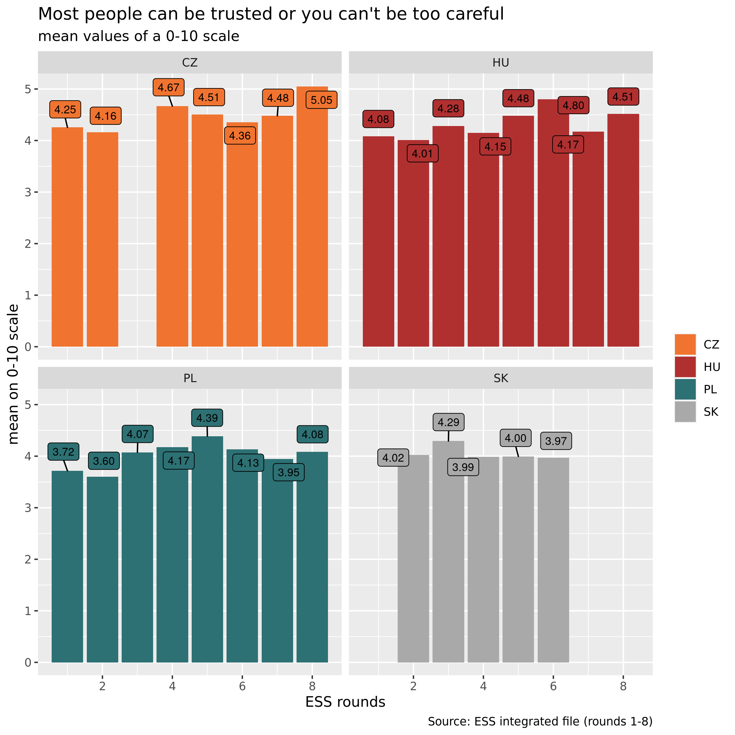
Than we prepare data with dplyr “verbs” and calculate unweighted means by cntry and essround.

d1 <- iess %>%
  select(ppltrst, cntry, essround) %>%
  group_by(cntry, essround) %>%
  summarise(ppl_mean = mean(as.numeric(ppltrst), na.rm = TRUE))
pandoc.table(head(d1))

-----------------------------
 cntry   essround   ppl_mean
------- ---------- ----------
  CZ        1        4.254
  CZ        2        4.163
  CZ        4        4.668
  CZ        5        4.506
  CZ        6        4.357
  CZ        7        4.479
-----------------------------

The plots will be drawn by geom_col() which uses values (such as “mean”, “sd”, whatever values) in d1 dataframe (ie. “stat_identity”) rather than number of cases (using “stat_count”). See details here. There will be four facets (sub-plots) for each country.

# Labels
ppl_tit <- attr(iess$ppltrst, "label")
subt <- "mean values of a 0-10 scale"
capt <- "Source: ESS integrated file (rounds 1-8)"
xl <- "ESS rounds"
yl <- "mean on 0-10 scale"
# Colors
my_cols <- c("#F07430", "#B03030", "#2D7174", "darkgrey")
p1 <- d1 %>%
  ggplot(aes(x = essround,
             y = ppl_mean,
             label = format(round(d1$ppl_mean, 2), nsmall = 2),
             fill = cntry)) +
    geom_col() +
    # remove letter 'a' from legend key
    geom_label_repel(show.legend = FALSE, vjust = -0.5) +
    scale_fill_manual(name = NULL, values = my_cols) +
    facet_wrap(~ cntry)
p1 <- p1 + labs(title = ppl_tit,
         subtitle = subt,
         caption = capt,
         x = xl,
         y = yl
         )
p1 <- p1 + theme(text = element_text(size = 16,  family = "Ubuntu Mono"))
p1

Unweighted means of generalized trust in V4 countries, 2002-2016

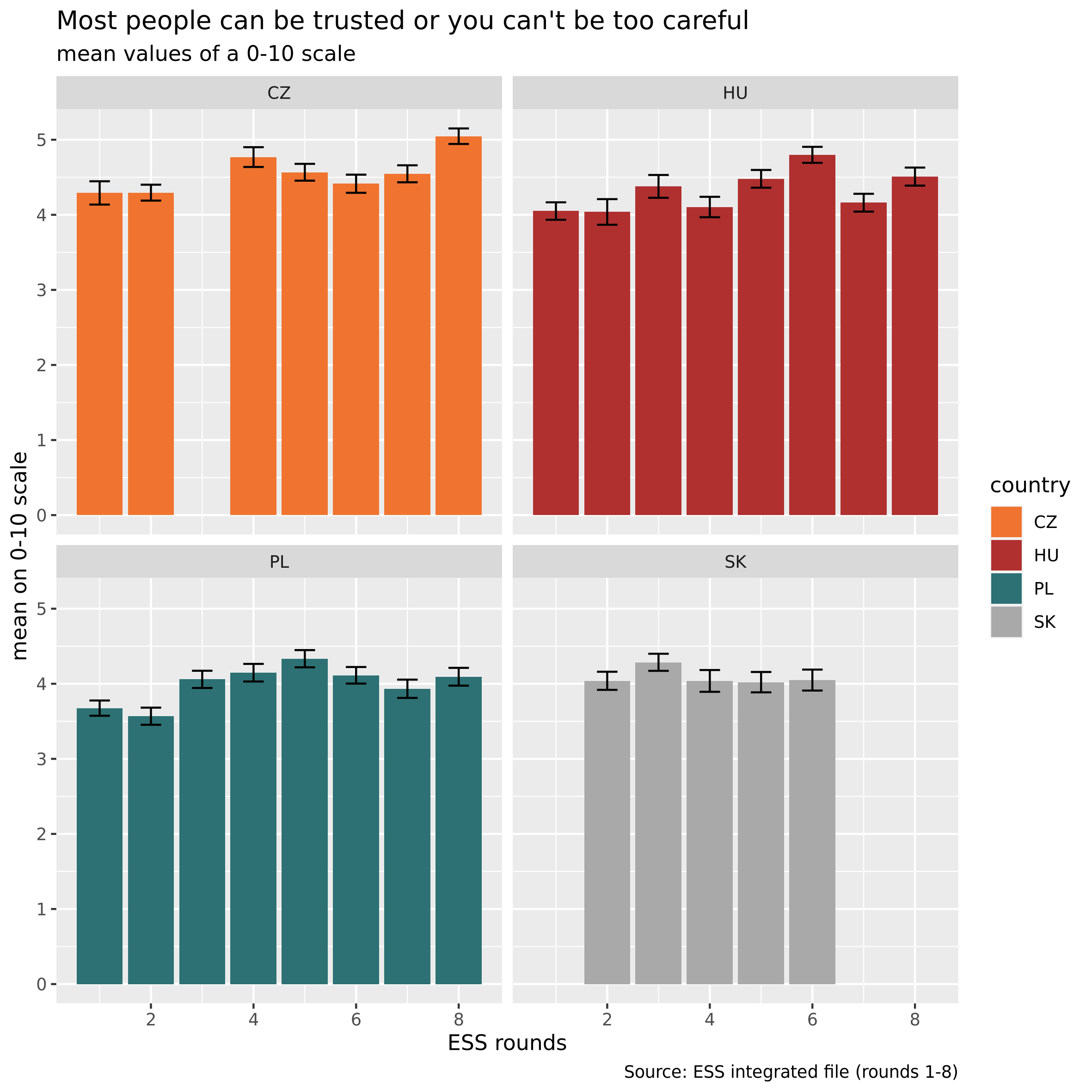
d1w <- iess %>%
  as_survey(weights = c(pspwght)) %>%
  select(ppltrst, cntry, essround) %>%
  group_by(cntry, essround) %>%
  summarise(ppl_wmean = survey_mean(as.numeric(ppltrst),
                                    na.rm = TRUE, vartype = "ci"))
pandoc.table(head(d1w))

--------------------------------------------------------------
 cntry   essround   ppl_wmean   ppl_wmean_low   ppl_wmean_upp
------- ---------- ----------- --------------- ---------------
  CZ        1         4.292         4.136           4.447
  CZ        2         4.295         4.189           4.401
  CZ        4         4.769         4.637           4.901
  CZ        5         4.567         4.455           4.679
  CZ        6         4.414         4.293           4.535
  CZ        7         4.546         4.433           4.66
--------------------------------------------------------------

p2 <- d1w %>%
  ggplot(aes(x = essround,
             y = ppl_wmean,
             ymin = ppl_wmean_low,
             ymax = ppl_wmean_upp,
             label = format(round(d1w$ppl_wmean, 1), nsmall = 1),
             fill = cntry)) +
    geom_col() +
    geom_errorbar(width = 0.4) +
    scale_fill_manual(name = "country", values = my_cols) +
    facet_wrap(~ cntry)

p2 <- p2 + labs(title = ppl_tit,
         subtitle = subt,
         caption = capt,
         x = xl,
         y = yl
         )
p2 <- p2 + theme(text = element_text(family = "Ubuntu Mono"))

1. Amelia McNamara: R Syntax Comparison:: CHEAT SHEET ↩

2. “The philosophy of the tidyverse is similar to and inspired by the “unix philosophy” (Raymond 2003), a set of loose principles that ensure most command line tools play well together.” Ross Z, Wickham H, Robinson D. 2017. Declutter your R workflow with tidy tools. PeerJ Preprints 5:e3180v1 https://doi.org/10.7287/peerj.preprints.3180v1 ↩