Adding capitals to “Eurostat-countries”

One can easily draw a map for 37 “Eurostat countries” as it was demonstrated in this post. However adding capital cities to the map can be tricky. The following example will use {maps} package for this purpose. The data at hand needs to be updated and cleaned to reflect recent political changes.

Steps:

1. Download the Eurostat map on NUTS 0 level (to draw country borders only and to omit subregions),

sf <- get_eurostat_geospatial(output_class = "sf", resolution = "60",
                              nuts_level = "0")

1. then add English country names to {eurostat} geospatial data using {countrycode} countrycode() function.

sf$country <- countrycode(sf$CNTR_CODE, origin="eurostat", 
                          destination = "country.name")

1. Next comes the data cleaning part. We use world.cities data from {maps}. This data contains the name of the capitals, latitude and longitude codes, plus population size data. Even after appropriate filtering the two data frames having different row numbers. Check with ?setdiff:

setdiff(sf$country, capseu$country.etc)
# [1] "Czechia"         "Montenegro"      "North Macedonia" "Serbia"         
# [5] "United Kingdom" 

It is because (1) Czech Republic name changed to Czechia, (2) “Serbia and Montenegro” became “Serbia” and “Montenegro” and have different capitals, and (3) “UK” in world.cities data should be recoded to “United Kingdom”. Even after these steps row numbers are still different. Solution: remove duplicates of Nicosia (as North-Cyprus is not recognized by the EU, and has the same capital with Cyprus).

1. Next, join filtered and cleaned world.cities data to Eurostat. Be sure that the resulted geospatial data preserving sf class

capitals_eu <- left_join(sf, capseu, by=c("country"))

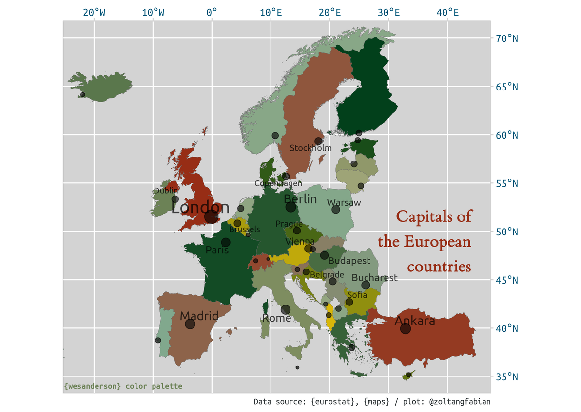
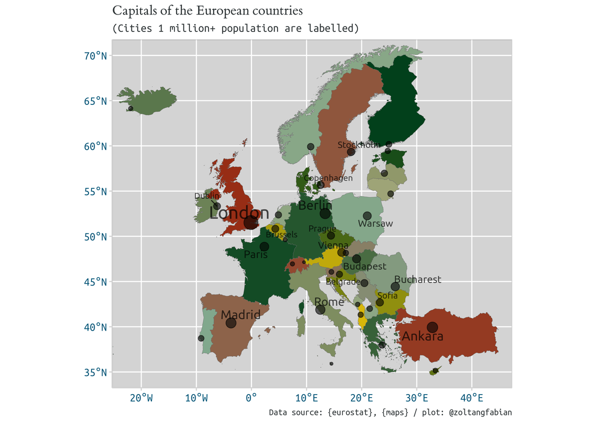
1. and plot the map with two layers: geom_sf() for countries and geom_points() for capitals.

p1 <- capitals_eu %>%
  ggplot(aes(fill = country)) +
  scale_fill_manual(values = pal) +
  geom_sf(color = "dim grey", size = .1) +
  geom_point(aes(x = long, y = lat, size = pop),
             color = "black", alpha = 0.6)

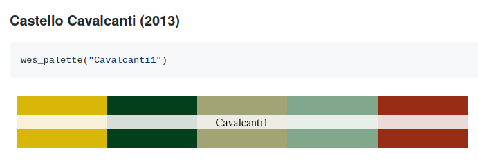
1. Add a custom style and a wes_anderson palette. A continuous palette can be generate like this:

# ?wes_palette
pal <- wes_palette("Cavalcanti1", 37, type = "continuous")

The example above & the result presented below used Cavalcanti1 palette, from the 2013 short film, Castello Cavalcanti.

1. Further aesthetics can be added via geom_text mapping to population size:

ggrepel::geom_text_repel(data = capseu, aes(x = long,
                                            y = lat,
                                            size = pop,
                                            label = labs,
                                            family = "Ubuntu"),
                              color = "black", alpha = 0.7) +
  guides(size= FALSE)

Result:

Resources:

• R source code
• Capitals of 37 European countries csv file