Getting started with Python pandas
What to do with Python’s pandas library?
Pandas is a fast, powerful, flexible and easy to use open source data analysis and manipulation tool, built on top of the Python programming language.
Ask Python itself what is pandas!
import pandas
pandas?
Here is some of the output:
pandas is a Python package providing fast, flexible, and expressive data structures designed to make working with “relational” or “labeled” data both easy and intuitive. It aims to be the fundamental high-level building block for doing practical, real world data analysis in Python. Additionally, it has the broader goal of becoming the most powerful and flexible open source data analysis / manipulation tool available in any language. It is already well on its way toward this goal.
Main Features
“Here are just a few of the things that pandas does well:
- Easy handling of missing data in floating point as well as non-floating point data.
- Size mutability: columns can be inserted and deleted from DataFrame and higher dimensional objects
- Automatic and explicit data alignment: objects can be explicitly aligned
to a set of labels, or the user can simply ignore the labels and let
Series,DataFrame, etc. automatically align the data for you in computations. - Powerful, flexible group by functionality to perform split-apply-combine operations on data sets, for both aggregating and transforming data.” (…)
Want to know more? Run pandas??! To save some typing pandas can be imported as pd like import pandas as pd. So pd?? will do it as well.
Go on with some real world example…
We shall import os, plotly (as plotly.express) and pandas and load our example gapminder dataset as DataFrame.
Now we import os, plotly (as plotly.express) and pandas modules than load our example gapminder dataset as DataFrame. Note: that this intro example is created as a jupyter-lab notebook, that is also exported to a python script. Results were exported to markdown and pdf. In order to render markdown correctly in Jekyll, some minor modification were needed. See the modified markdown file on github.
import os
import plotly.express as px
import pandas as pd
df = px.data.gapminder()  # n.b. there is a separate module for gapminder data
type(df)
pandas.core.frame.DataFrame
Have a look at some attributes and descriptive statistics of our DataFrame.
df.head(5)
| country | continent | year | lifeExp | pop | gdpPercap | iso_alpha | iso_num | |
|---|---|---|---|---|---|---|---|---|
| 0 | Afghanistan | Asia | 1952 | 28.801 | 8425333 | 779.445314 | AFG | 4 |
| 1 | Afghanistan | Asia | 1957 | 30.332 | 9240934 | 820.853030 | AFG | 4 |
| 2 | Afghanistan | Asia | 1962 | 31.997 | 10267083 | 853.100710 | AFG | 4 |
| 3 | Afghanistan | Asia | 1967 | 34.020 | 11537966 | 836.197138 | AFG | 4 |
| 4 | Afghanistan | Asia | 1972 | 36.088 | 13079460 | 739.981106 | AFG | 4 |
df.shape #without parents!
(1704, 8)
pd.set_option('display.float_format', lambda x: '%.1f' % x)  # set number of digits
df.describe()
| year | lifeExp | pop | gdpPercap | iso_num | |
|---|---|---|---|---|---|
| count | 1704.0 | 1704.0 | 1704.0 | 1704.0 | 1704.0 |
| mean | 1979.5 | 59.5 | 29601212.3 | 7215.3 | 425.9 |
| std | 17.3 | 12.9 | 106157896.7 | 9857.5 | 248.3 |
| min | 1952.0 | 23.6 | 60011.0 | 241.2 | 4.0 |
| 25% | 1965.8 | 48.2 | 2793664.0 | 1202.1 | 208.0 |
| 50% | 1979.5 | 60.7 | 7023595.5 | 3531.8 | 410.0 |
| 75% | 1993.2 | 70.8 | 19585221.8 | 9325.5 | 638.0 |
| max | 2007.0 | 82.6 | 1318683096.0 | 113523.1 | 894.0 |
df["country"].value_counts()
Nicaragua           12
Gambia              12
Rwanda              12
Cambodia            12
Congo, Dem. Rep.    12
                    ..
Sudan               12
Swaziland           12
Peru                12
Bulgaria            12
Costa Rica          12
Name: country, Length: 142, dtype: int64
Filtering DataFrame
- Select the most recent year.
df["year"].max()
2007
Exclude all previous years and keep 2007 only with a query.
df.query('year == 2007')
| country | continent | year | lifeExp | pop | gdpPercap | iso_alpha | iso_num | |
|---|---|---|---|---|---|---|---|---|
| 11 | Afghanistan | Asia | 2007 | 43.8 | 31889923 | 974.6 | AFG | 4 |
| 23 | Albania | Europe | 2007 | 76.4 | 3600523 | 5937.0 | ALB | 8 |
| 35 | Algeria | Africa | 2007 | 72.3 | 33333216 | 6223.4 | DZA | 12 |
| 47 | Angola | Africa | 2007 | 42.7 | 12420476 | 4797.2 | AGO | 24 |
| 59 | Argentina | Americas | 2007 | 75.3 | 40301927 | 12779.4 | ARG | 32 |
| ... | ... | ... | ... | ... | ... | ... | ... | ... |
| 1655 | Vietnam | Asia | 2007 | 74.2 | 85262356 | 2441.6 | VNM | 704 |
| 1667 | West Bank and Gaza | Asia | 2007 | 73.4 | 4018332 | 3025.3 | PSE | 275 |
| 1679 | Yemen, Rep. | Asia | 2007 | 62.7 | 22211743 | 2280.8 | YEM | 887 |
| 1691 | Zambia | Africa | 2007 | 42.4 | 11746035 | 1271.2 | ZMB | 894 |
| 1703 | Zimbabwe | Africa | 2007 | 43.5 | 12311143 | 469.7 | ZWE | 716 |
142 rows × 8 columns
We got a df with 142 rows which is equal to the number of countries. And this is so True.
len(df.country.unique()) == len(df.query('year == 2007'))
True
Which country has the lowest life expectancy in Europe in 2007? First print the value.
df.query('year == 2007 & continent == "Europe"')["lifeExp"].min()
71.777
What country has the highest life expectancy worldwide?
maxLE = df['lifeExp'].max()
df[df['lifeExp'] == maxLE]
| country | continent | year | lifeExp | pop | gdpPercap | iso_alpha | iso_num | |
|---|---|---|---|---|---|---|---|---|
| 803 | Japan | Asia | 2007 | 82.603 | 127467972 | 31656.06806 | JPN | 392 |
What country has the highest life expectancy in each continent?
df.groupby("continent").max("lifeExp")
| year | lifeExp | pop | gdpPercap | iso_num | |
|---|---|---|---|---|---|
| continent | |||||
| Africa | 2007 | 76.442 | 135031164 | 21951.21176 | 894 |
| Americas | 2007 | 80.653 | 301139947 | 42951.65309 | 862 |
| Asia | 2007 | 82.603 | 1318683096 | 113523.13290 | 887 |
| Europe | 2007 | 81.757 | 82400996 | 49357.19017 | 826 |
| Oceania | 2007 | 81.235 | 20434176 | 34435.36744 | 554 |
df.groupby(['continent'], sort=False)['lifeExp'].max()
continent
Asia        82.603
Europe      81.757
Africa      76.442
Americas    80.653
Oceania     81.235
Name: lifeExp, dtype: float64
Well, mission completed, but we are still lack the name of the countries :-( So copy paste from here.
idx = df.groupby(['continent'])['lifeExp'].transform(max) == df['lifeExp']
df[idx]
| country | continent | year | lifeExp | pop | gdpPercap | iso_alpha | iso_num | |
|---|---|---|---|---|---|---|---|---|
| 71 | Australia | Oceania | 2007 | 81.235 | 20434176 | 34435.367440 | AUS | 36 |
| 251 | Canada | Americas | 2007 | 80.653 | 33390141 | 36319.235010 | CAN | 124 |
| 695 | Iceland | Europe | 2007 | 81.757 | 301931 | 36180.789190 | ISL | 352 |
| 803 | Japan | Asia | 2007 | 82.603 | 127467972 | 31656.068060 | JPN | 392 |
| 1271 | Reunion | Africa | 2007 | 76.442 | 798094 | 7670.122558 | REU | 638 |
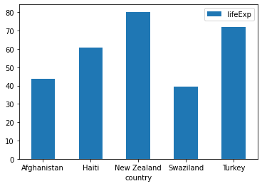
Now, look at the minimum values by continent! But remember to filter for the most recent data.
df2 = df.query('year == 2007')
idx = df2.groupby(['continent'])['lifeExp'].transform(min) == df2['lifeExp']
df2[idx]
| country | continent | year | lifeExp | pop | gdpPercap | iso_alpha | iso_num | |
|---|---|---|---|---|---|---|---|---|
| 11 | Afghanistan | Asia | 2007 | 43.828 | 31889923 | 974.580338 | AFG | 4 |
| 647 | Haiti | Americas | 2007 | 60.916 | 8502814 | 1201.637154 | HTI | 332 |
| 1103 | New Zealand | Oceania | 2007 | 80.204 | 4115771 | 25185.009110 | NZL | 554 |
| 1463 | Swaziland | Africa | 2007 | 39.613 | 1133066 | 4513.480643 | SWZ | 748 |
| 1583 | Turkey | Europe | 2007 | 71.777 | 71158647 | 8458.276384 | TUR | 792 |
Ta da! It is Turkey that had the lowest life expectancy in Europe according to the example dataset.
Finally, a quick plot of the results with Pandas-only way (i.e. we shall not use plotly’s advanced capabilities).
ax = df2[idx].plot.bar(x='country', y='lifeExp', rot=0)