Data wrangling is the process of shaping data into a format that is appropriate for specific analytical purposes. In the following example we shall read John Hopkins University’s (JHU) COVID-19 deaths database. It contains daily cumulative number of COVID-19 deaths for countries, and in some cases (like USA) for provinces/states. Our focus is the four Visegrad (V4) countries (i.e. Czechia, Hungary, Poland and Slovakia). Each V4 country represented by a single row in the database.
Let’s read the data with read_csv function, that is part of tidyverse package(s) - namely readr. It will create a tibble, which is a “modern” form of data.frame.
uri <- c("https://raw.githubusercontent.com/CSSEGISandData/COVID-19/master/csse_covid_19_data/csse_covid_19_time_series/time_series_covid19_deaths_global.csv")
df <- read_csv(uri)
df
       `Province/State` `Country/Region`   Lat   Long
       <chr>            <chr>            <dbl>  <dbl>
     1 <NA>             Afghanistan       33.9  67.7
     2 <NA>             Albania           41.2  20.2
     3 <NA>             Algeria           28.0   1.66
     4 <NA>             Andorra           42.5   1.52
     5 <NA>             Angola           -11.2  17.9
     6 <NA>             Antigua and Bar…  17.1 -61.8
     7 <NA>             Argentina        -38.4 -63.6
     8 <NA>             Armenia           40.1  45.0
     9 Australian Capi… Australia        -35.5 149.
    10 New South Wales  Australia        -33.9 151.
As you can see Australia is represented by more than one Province/State, while some other (smaller) countries only by one. So, in case of need one should aggregate data to country-level. We, shall skip this step.
There are 266 rows (states) that is 188 unique countries (cf. unique(df$'Country/Region'). We also have 180 “day-date” columns, but we want to have only one for each values in long format.
Before doing the actual pivoting, drop and rename some of the columns we don’t need:
df <- df %>% select(-c("Province/State", "Lat", "Long"))
df <- df %>% rename(c("country" = "Country/Region"))
Select V4 rows by filtering:
v4 <- c("Hungary", "Slovakia", "Poland", "Czechia")
df <- df %>% filter(country %in% v4)
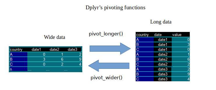
Use pivot_longer tidyr function to do the actual transformation. (It does the same as the legacy function gather, but in somewhat simpler and more straightforward manner.)
# switch to long format, so each date column parsed to one column
df <- pivot_longer(df, cols = ends_with("20"),
    names_to = "date", values_to = "deaths")
Voila:
A tibble: 720 x 3
  country date    deaths
  <chr>   <chr>    <dbl>
1 Czechia 1/22/20      0
2 Czechia 1/23/20      0
Notice that we used cols=ends_with, but there are several other ways to identify columns to be gathered. Other options for tidy-select argument are listed in reference.
We shall convert date column from character <chr> to date <date> format, and arrange rows by date and country.
  df$date <- as.Date(df$date, "%m/%d/%y")
  df <- arrange(df, date, country)
  tail(df)
A tibble: 6 x 3
  country  date       deaths
  <chr>    <date>      <dbl>
1 Poland   2020-07-18   1618
2 Slovakia 2020-07-18     28
3 Czechia  2020-07-19    359
4 Hungary  2020-07-19    596
5 Poland   2020-07-19   1624
6 Slovakia 2020-07-19     28
Next we can easily filter our columns based on date values like this: df %>% filter(date >= "2020-06-14"). The long format has an advantage of being more usable with ggplot package.
Data from long to wide format can be easily switched back with pivot_wider function:
dfw <- df %>% pivot_wider(names_from = date, values_from = deaths)
We have 4 rows (V4 countries) and 176 columns (175 time-points). Limits on time-range with select function can be added, and ``select` accepts position intervals as well.
dfw <- dfw %>% select(1, 146:176)
Finally write our df as RDS data for further use. You may want to download from here.
saveRDS(df, file = "v4_c19_d_200720.RDS")
That’s all for now. Next we shall create a multi-line chart with ggplot. Check out here.
- Download the whole .R script
- Cf. tidyr 1.0.0 is here. pivot_longer & pivot_wider replace spread & gather
- What is tidy data? (Hadley Wickham - ViennaR Meetup March 2019)